Page 10

As for the linear fit, the quadratic or parabolic fit is discontinuous. Yet it is

possible after the fact to take advantage of the overlap between the series of fitted curves
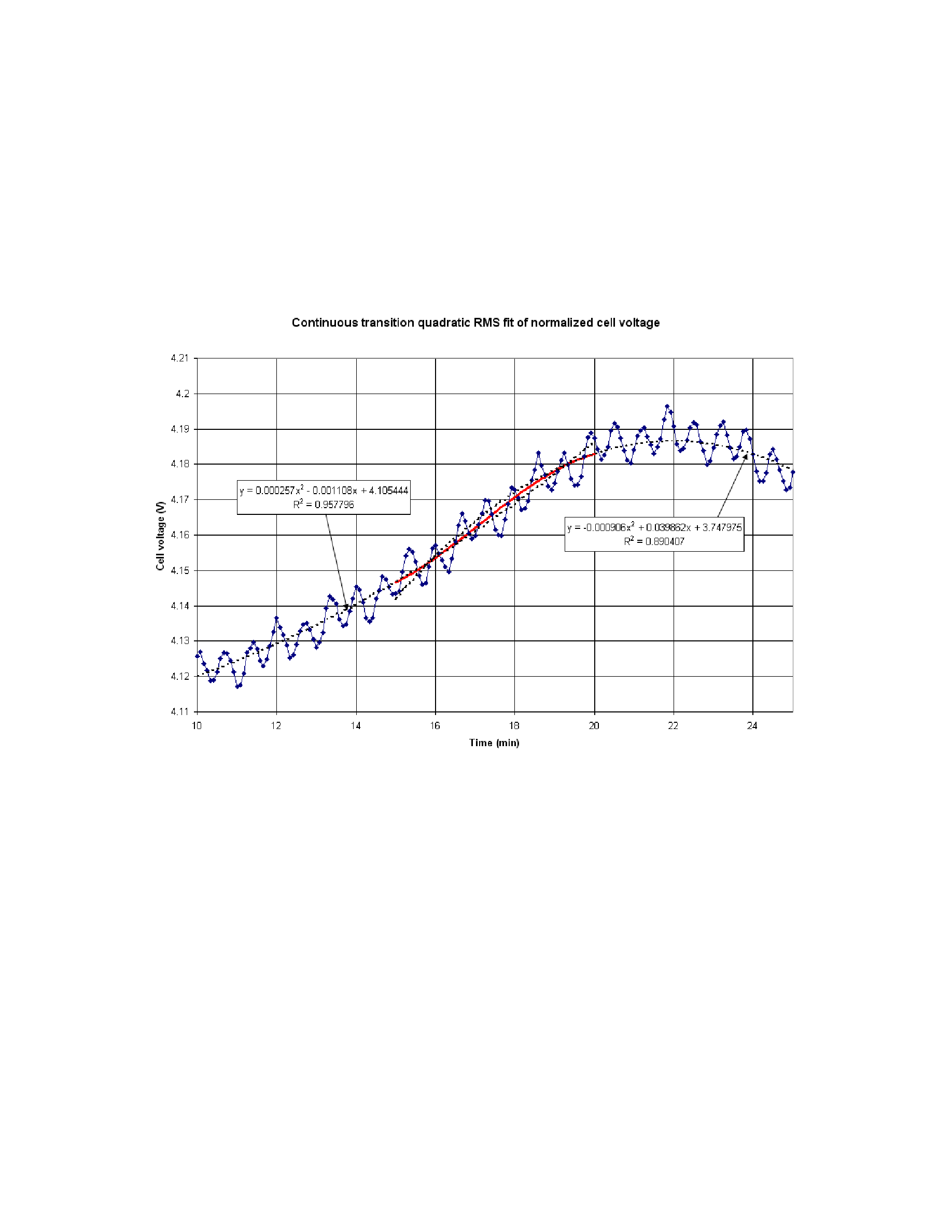
to produce a single continuous curve by doing some interpolation. For example, the red
curve in Figure 11 is produced by interpolating between the two overlapping fitted
curves in the 15 to 20 minutes time segment. The interpolation is done is such a way that
even the first derivative of the curve is continuous between time segments.

Figure 11: Continuous transition quadratic RMS fit of normalized cell voltage

Repeating this procedure from time segment to time segment produced the red

curve presented in Figure 12. Evidently, this after-the-fact treatment is not helping
improving the slope estimation at the end of the last available segment which is the
current time when the information is required to take control actions as part of the cell
control logic.

Yet, at least this red curve in Figure 12 can now be compared to the equivalent of

the blue curve in Figure 4 to determine the appropriateness of the selected curve fitting
algorithm.