So clearly even if the 5 cycles are not identical, they almost perfectly match a
which corresponds to the typical range the In Situ controller would be able to operate the
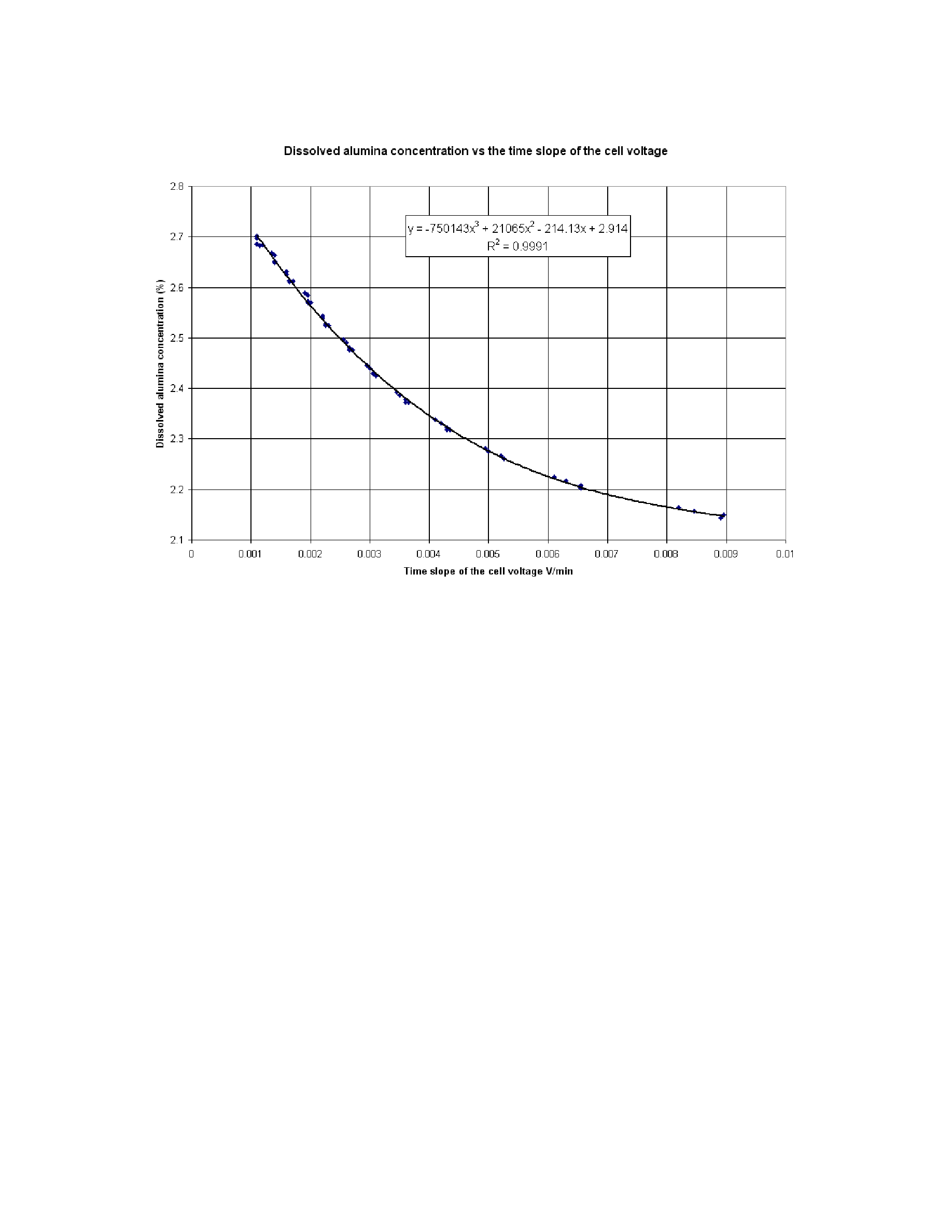
cell and for a different value of the alumina dissolution constant, the linear correlation
presented in Figure 16 was obtained. This is the correlation that will be used to estimate
the alumina concentration once the slope of the noise free normalized cell voltage have
been estimated by the In Situ controller in Dyna/Marc test runs.
For example, the slope of 3.9 mV/min estimated after 10 minutes of no feed
concentration of:
-0.0279 * 3.9 + 2.3193 = 2.21 %
Using the correlation of Figure 15 would lead to a different estimate:
-750143 * 0.0039
This 0.14 % discrepancy between the real alumina concentration and the
simply introduce a 0.14% offset on the targeted alumina concentration.