Abstract
In the present study, the full 3D thermo-electric model of a 500 kA demonstration cell has been weakly coupled with the non-linear wave MHD model of the full version of the same cell.
In the MHD model, the horizontal ledge distribution calculated in the thermo-electric model has been incorporated as part of the model geometry.
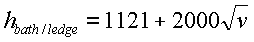
In the thermo-electric model, the velocity fields calculated by the MHD model in both the bath and the metal have been used to setup the local heat transfer coefficients at the liquids/ledge interface.
Both models have been solved alternatively until a convergence for the horizontal ledge distribution has been obtained.
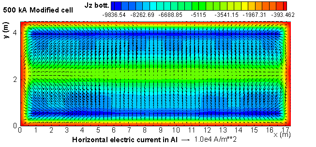
The MHD model has been upgraded with the transiently coupled ferromagnetics solution module, ledge input and with an optimized bus-bar arrangement for a stable 500 kA cell suitable for commercial application.
Introduction
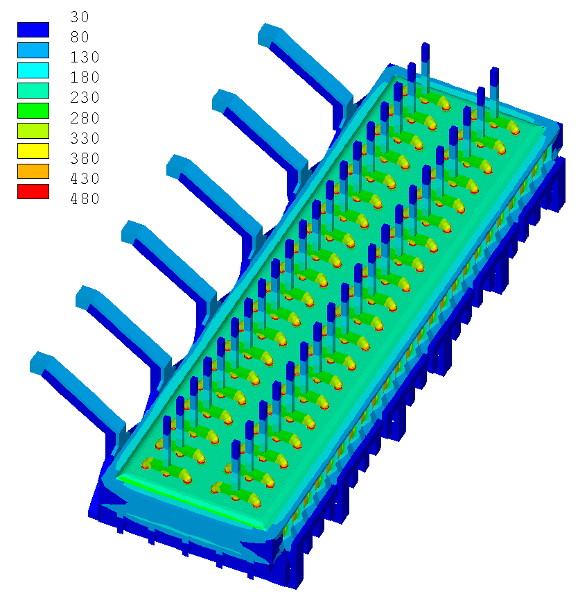
The mesh of a 3D full cell and external bus-bar thermo-electric model of a 300 kA cell has been presented in 2002 (see figure 10 of [1]). That 423,296 element model could not be solved on the PIII computer available to the author at the time.
More recently, the mesh of a 3D full cell and external bus-bar thermo-electric model of a 500 kA cell has been presented (see figure 6 of [2]). That 585,016 element model could not be solved either, even on a P4 3.2 GHz computer with 2 GB of RAM.
Yet, this is the type of thermo-electric model that the authors want to couple with the non-linear wave MHD model [3, 2] in order to be able to take into consideration the interactions between the thermo-electric and the MHD aspects of the cell behavior [4].
Perseverance finally pays off as these two models could finally be solved. For the first time, the results of those two 3D full cell and external bus-bar thermo-electric models will be presented.
3D full cell and external bus-bar thermo-electric model of the 300 kA demonstration model
Since this very first 3D full cell and external bus-bar thermo-electric 423,296 elements model has been built on a PIII computer having only 384 MEG of RAM [1], it has not even been considered to try to solve it on that hardware.
Later on, when the P4 computer with 2GB became available, a bigger 500 kA cell demonstration model was build and the attempt to solve it failed [2].
Taking a step back, it is now possible to attempt to solve the 300 kA cell model on that same P4 computer. It is even possible to take a second step back and try instead to solve a coarser mesh version of that same 300 kA cell model.
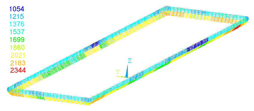
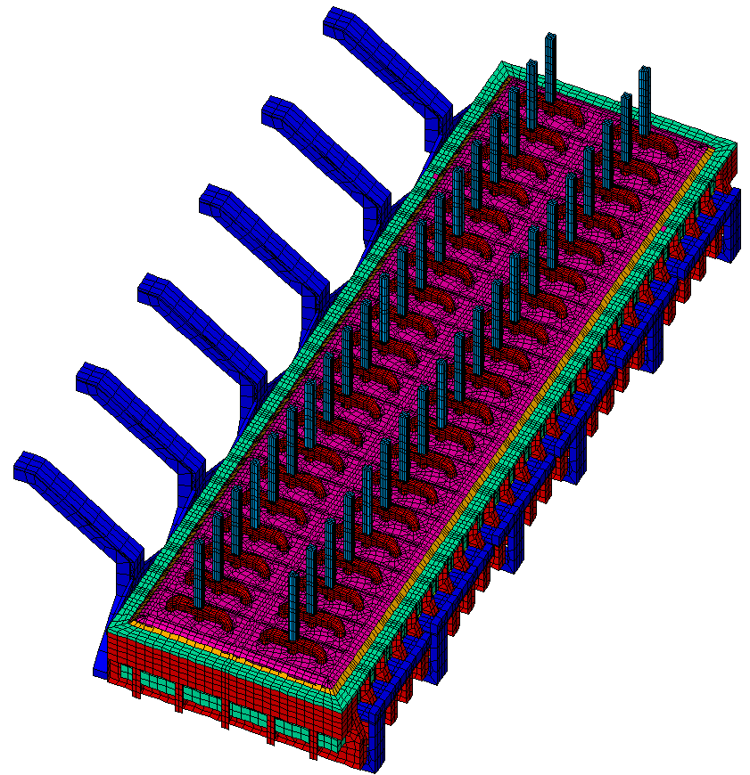
Figure 1: Coarser mesh of the 3D full cell and external bus-bar thermo-electric 300 kA cell model.

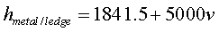 (1)
(1)
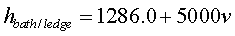 (2)
(2)
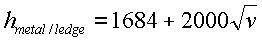 (3)
(3)
 (4)
(4)